2. Reference guide¶

2.1. TimeSeries¶

2.1.1. Some terminology¶

data value: single, scalar value recorded at a specific time
data samples:one or more values associated with a specific time. number of data samples in a time series is the same as thr length of the time vector

2.1.2. todo¶

2.1.2.1. Methods to implement in timeseries¶

addsample Add a data sample to a timeseries object.
append Concatenate timeseries objects in the time dimension.
delsample Delete a sample from a timeseries object.
detrend Subtract the mean or best-fit line and remove all NaNs from time-series data.
filter Shape frequency content of time-series data using a 1-D digital filter.
getinterpmethod Get the interpolation method for a timeseries object.
getsampleusingtime Extract data samples from an existing timeseries object into a new timeseries object based on specified start and end time values.

idealfilter Apply an ideal pass or notch (noncausal) filter to a timeseries object.

resample elect or interpolate data in a timeseries object using a new time vector.
setinterpmethod et interpolation method for a timeseries object.
synchronize Synchronize and resample two timeseries objects using a common time vector.

class Event(date=None, text=None, value=None, short_text=None)¶

Event class

>>> import datetime
>>> d1 = datetime.datetime(2000, 1, 1)
>>> event = Event(d1, "event 1", 10)
>>> event.value
10

class Events¶

List of events

Inherits from dict. Simply check that the object added is an instance of Event.

Each key is either a from event.short_text or from a counter.

2 methods to remove or get elements that are just aliases to del and get method of dictionary class.

>>> import datetime
>>> import datetime
>>> d1 = datetime.datetime(2000, 1, 1)
>>> event1 = Event(d1, "event 1", 10, 'ev1')
>>> d2 = datetime.datetime(2000, 10, 1)
>>> event2 = Event(d2, "event 2", 10, 'ev2')
>>> events = Events()
>>> events.addevent(d1)
>>> events.addevent(d2)
>>> del events['ev1']
>>> events.keys()
['ev2']

addevent(event)¶

class TSCollections¶

add_timeseries(ts)¶

class TimeRange(start, end, num=None, step=None, frequency=None)¶: d1 = datetime.datetime(2010,1,1) d2 = datetime.datetime(2010,2,1)

class TimeSeries(data, name=None, time=None, units=None, step=1, events=None, dataquality=None, interpolation=None, start=None, end=None, frequency=None)¶

TimeSeries stores data and time vectors.

The time vector length (if provided) must be the same as data vector. If the time values are date strings, you must specify Time as a cell array of date strings.

If the time vector contains duplicate values:

Duplicated values must occupy contiguous elements.

Time values must not be decreasing.

Interpolating time-series data using methods like resample and synchronize can produce different results depending on whether the input timeseries contains duplicate times.

Default: A time vector that ranges from 0 to N-1 with a 1-second interval, where N is the number of samples. In such case, the time vector is said to be relative. If startdate is provided, then it is absolute.

The attribute data contains a wrapping version of the input parameter data into a numpy.array So, data contains all methods provided by numpy.array. For example, data.mean(). However, we creates attributes for some of the standard descriptive statistics. So:
>>> ts = TimeSeries([1,2,0,1])
>>> ts.mean
2.
is equivalent to:
>>> ts = TimeSeries([1,2,0,1])
>>> ts.mean()
2.
>>> ts = TimeSeries([-1,1,-2,2,5])
>>> ts.time
[0,1,2,3,4]
>>> ts.mean
1.0
In addition to data and time values, you can also use the time-series object to store events, descriptive information about data and time, data quality, and the interpolation method.

Data Sample

if start and end are not provided, time range is (0, N*step, N) if start is provided but not end, time range is (start, start+step*N, N) if start and end provided, time range is (start, end, N)

N¶: data sample size

addSample(data)¶

data¶

getData()¶

getDataSampleSize()¶

getIQR()¶

getMAX()¶

getMEAN()¶

getMEDIAN()¶

getMIN()¶

getN()¶

getSTD()¶

getVAR()¶

gettsafteratevent(label)¶: Create a new timeseries object by extracting the samples from an existing time series that occur after or at a specified event.

gettsatevent()¶: Create a new timeseries object by extracting the samples that occur at the same time as a specified event from an existing time series.

gettsbeforeatevent(label)¶: gettsbeforeevent Create a new timeseries object by extracting the samples that occur before a specified event from an existing time series.

See also

gettsbetweenevents()

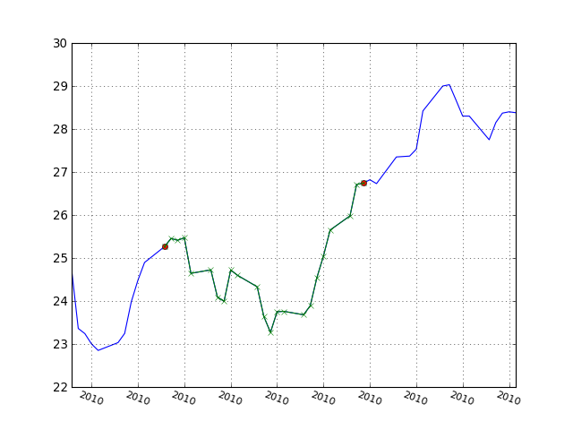
gettsbetweenevents(label1, label2)¶

Create a new timeseries object by extracting the samples that occur between two specified events from an existing time series.

from timeseries import *
d1 = datetime.datetime(2010,1,1)
d2 = datetime.datetime(2011,1,1)
fd = FinancialData('MT.PA', d1, d2)

t1 = TimeSeries(fd.data.low, time=fd.data.date)
event1 = Event(datetime.datetime(2010, 11, 8), "event1", t1.data[10], "ev1")
event2 = Event(datetime.datetime(2010, 12, 8), "event2", t1.data[32], "ev2")
t1.events.addevent(event1)
t1.events.addevent(event2)

t1.plot()
t2 = t1.gettsbetweenevents('ev1', 'ev2')
t2.plot('xg-', keep=True)  # to not erase the previous plot

[hires.png, pdf]

hist(bins=10)¶: Simple histogram using pylab.hist

iqr¶: Return the iqr of timeseries data.

max¶: Return the maximum value of timeseries data.

mean¶: Return the mean of timeseries data.

median¶: Return the median of timeseries data.

min¶: Return the minimum value of timeseries data.

plot(*args, **kargs)¶

kargs withevents bool

events_properties todo

setData(data)¶

std¶: Return the standard deviation of timeseries data.

step¶

var¶: Return the var of timeseries data.

addmonth(date)¶

ar(values, errors, alpha)¶: An autoregressive time series process has the following form:

$y_t = \alpha_0 + \alpha_1 y_{t-1} + \dots + \alpha_n y_{t-n} + \epsilon_t$

arch(values, errors, alpha)¶: An autoregressive conditional heteroscedastic (ARCH) process has the following form

$y_t = \sigma_t \epsilon_t$

$\sigma_t = \alpha_0 + \alpha_1 y^2_{t-1} + \dots + \alpha_n y^2_{t-n}$

arma(values, errors, alpha, beta)¶

AR and MA processes can be combined to obtain an ARMA-process:

$y_t = \alpha_0 + \alpha_1 y_{t-1} + \dots + \alpha_n y_{t-n} + \beta_1 \epsilon_{t-1} + \dots + \beta_m\epsilon_{t-m} + \epsilon_t$

Such an ARMA time series can be created with the following code:

import numpy
n = 10
mu = 0
sig = 1
errors = numpy.random.normal(mu, sig, n)
n_ar = 3
alpha = numpy.random.uniform(0,1,n_ar)
n_ma = 2
beta = numpy.random.uniform(0,1,n_ma)
values = numpy.zeros(n)
arma(values, errors, alpha, beta)

garch(values, errors, alpha, beta)¶

GARCH provess

ARCH process can be extended to a general autoregressive conditional heteroscedastic (GARCH) process by incorporating also laged values of

$y_t = \sigma_t \epsilon_t$

$\sigma_t = \alpha_0 + \alpha_1 y^2_{t-1} + \dots + \alpha_n y^2_{t-n} + \beta_1 \sigma_{t-1} + \dots + \beta_m\sigma_{t-m} + \epsilon_t$

import numpy
import math
n = 10
mu = 0
sig = 1
errors = numpy.random.normal(mu, sig, n)
n_a = 2
alpha = numpy.random.uniform(0,1,n_a)
n_b = 2
beta = numpy.random.uniform(0,1,n_b)
values = numpy.zeros(n)
sigma2 = numpy.zeros(n)
garch(values, errors, alpha, beta)

ma(values, errors, beta)¶: A moving average time series process has the form:

$y_t = \beta_0 + \beta_1 \epsilon_{t-1} + \dots + \beta_n\epsilon_{t-n} + \epsilon_t$

timeConvertor(date)¶

Convert an input into a valid datetime instance.

If the input is already a datetime, just return it. If the input is a string, the format may be :

dd-mm-yyyy dd:mm:yyyy yyyy:mm:dd yyyy-mm-dd dd/mm/yyyy yyyy/mm/dd

Note that month is always between year and days.

>>> d1 = timeConvertor('2000-12-31')
>>> d2 = timeConvertor('31-12-2000')
>>> assert d1 == d2
True
>>> d1 = timeConvertor('2000:12:31')
>>> d2 = timeConvertor('2000/12/31')
>>> assert d1 == d2
True

2.2. Data sets¶

get_imcenfant_data()¶: #imcenfant.csv #Description Un echantillon de dossiers d’enfants a ete saisi. Ce sont des enfants vus lors d’une visite en 1ere section de maternelle en 1996-1997 dans des ecoles de Bordeaux (Gironde, France). L’echantillon est constitue de 152 enfants ages de 3 ou 4 ans. #tableau descriptif du jeu de donnees #sexe, f or g, #ecole situe en zone prioritaire oui (O) non (N) # poids # age annee # age mois # taille(cm)

get_m30_data()¶

fatalities on the road frequency of 30 days

Source :	[Aragon2010]

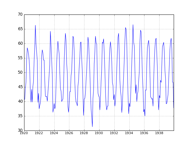
get_nottem_data()¶

from pylab import *
from timeseries import *
ts = get_nottem_data()
ts.plot()

[hires.png, pdf]

Source :	[Aragon2010]

get_popfr_data()¶

French population over time.

returns a TimeSeries instance

Source :	[Aragon2010]

2.3. Financial Data¶

class FinancialData(value, d1, d2)¶

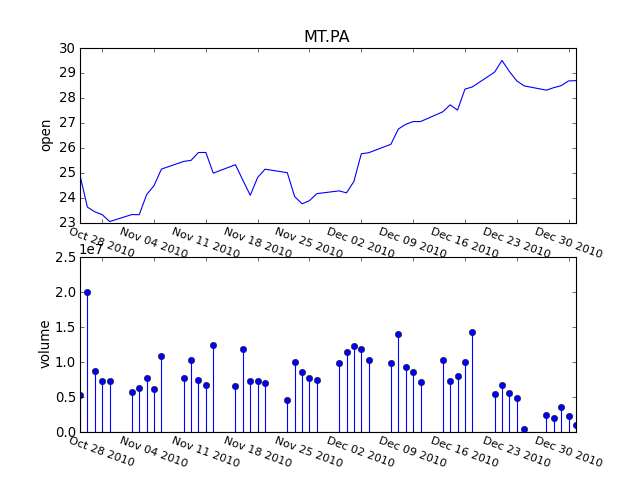
Class to get financial data and create summary plots.

import datetime
from timeseries import FinancialData
d1 = datetime.datetime(2010,1,1)
d2 = datetime.datetime(2011,1,1)
fd = FinancialData('MT.PA', d1, d2)
fd.plot_summary()

[hires.png, pdf]

Uses matplotlib.finance to get the data from yahoo.

Parameters:	value – a valid string e.g. “google”, ‘arcelor’, ... d1 – a valid datetime d2 – a valid datetime
Attributes :	d1, d2, value, data

data contains the volume, open, close, low and high values.

d1¶

d2¶

data¶

getD1()¶

getD2()¶

getDATA()¶

getReturns()¶

getValue()¶

get_finance_yahoo(adjusted=True)¶

Uses pylab tools to get yahoo finance data

Parameters:	adjusted (bool) – True see pylab doc

hist_returns(nbins=100)¶: plot the histogram of returns values and approximate normalised histogram

plot_returns(i=None, f=None, log=False)¶: plot the returns values

plot_summary()¶: Plot the open values and volumes.

plot_volume(*args, **kargs)¶: Plot the volume versus time

returns¶: returns the arithmetic returns (close-open()/open( to be checked

rotate_xticks(fontsize=10, rotation=0)¶

setD1(d1)¶

setD2(d2)¶

value¶

Front page|TimeSeries - Time Series Analysis in Python (0.2)

2. Reference guide¶

2.1. TimeSeries¶

2.1.1. Some terminology¶

2.1.2. todo¶

2.1.2.1. Methods to implement in timeseries¶

2.2. Data sets¶

2.3. Financial Data¶

Table Of Contents, Home

Search